- Computers are needed for lab this week
- Calculate the acceleration of a cart on an inclined track
- Conceptually, students find this experiment easier than the Conservation of Energy! However…
- … this experiment is after their first exam and usually October break, so they often forget everything they've learned so far about recording data and writing a lab report! You've been warned
- Tracks will be inclined at the same angle as in the Cons. of E. experiment
 Students will calculate a value of the acceleration from their graph that they compare to g·sinθ, calculated from their measurement of track angle, θ. Students will calculate a value of the acceleration from their graph that they compare to g·sinθ, calculated from their measurement of track angle, θ.
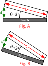
- There is frequently a disagreement here, since the angle is very small, and the uncertainty in the level of the table can overwhelm even the most careful measurement. A perfect opportunity to discuss measurement uncertainty!
- Example: Careful measurement of the track length and elevation gives an angle of 5° (Fig. A). However, if the table were tilted at 30° the true angle of the track could be anywhere from 25° to 35°! (Fig. B)
- Expected track angle results:
- Black tracks (A,B,C,D): d = 9.0 cm; L = 137.0 cm. So, θ = 3.77°, and g·sinθ = 64.4 cm/s2
- Black track note: Make sure the spring bumper is flipped up on the high end of the track so that the gold carts can start at the 25 cm mark
- Silver tracks (E,F,G,H): d = 9.0 cm; L = 180.5 cm. So, θ = 2.86°, and g·sinθ = 48.9 cm/s2
- Make sure that students calculate L as the difference between two measurements on all tracks!
- Photogate notes:
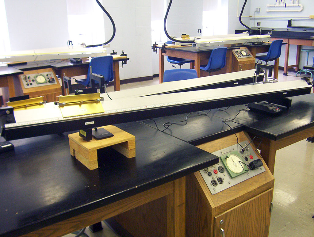
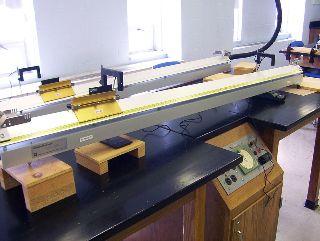
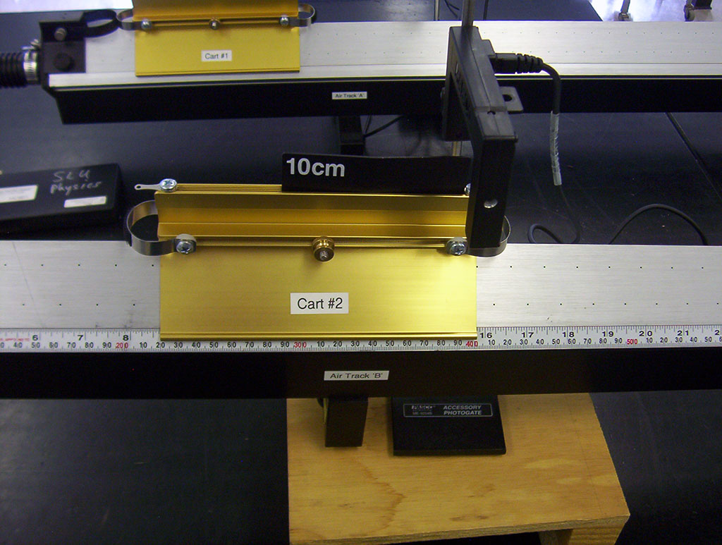
- This week, an accessory photogate is attached to the main photogate timer, so students will be recording the time it takes for the cart to travel between the two photogates: Photo #1 – Black Tracks; Photo #2 – Silver Tracks; Photo #3 – Photogate connection
- Black tracks: the accessory photogate sits on top of the wood platform used to raise the track; note that the flag will need to be moved to the front of the cart so that the timer can be tripped at 40 cm: see this photo
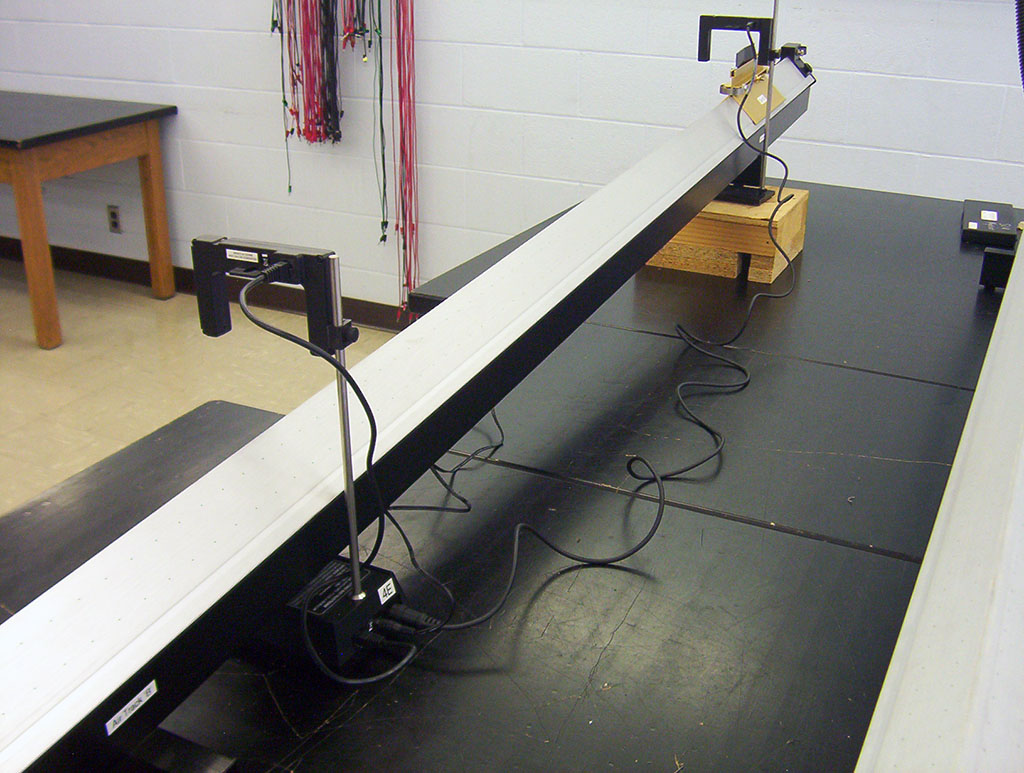
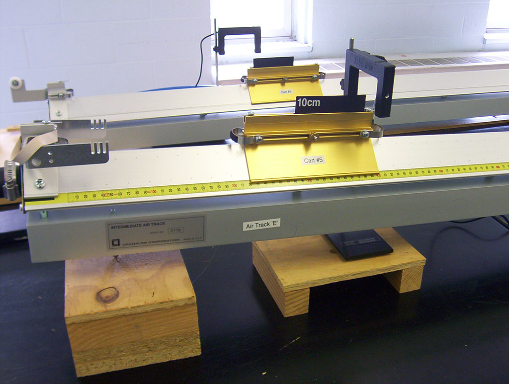
- Silver tracks: the accessory photogate sits on top of a second, lower wood platform: see this photo
- The photogates are positioned so that they are tripped when the front edge of the cart reaches a specific position on the track, the same as with the Cons. of E. experiment. Once again, the procedure in the instructions is necessary since the flag is not flush with the front edge of the cart. Some students may realize that the flag can be moved to the front edge of the cart. This is fine, but the flags on the carts they will use on the lab practical are fixed in place, so knowing the correct procedure is important. Don't tell them about the lab-practical carts, but ask what they would do if the cart was fixed in place. Some might try to measure the offset, which is a lot harder and will introduce more error than just following the instructions!
- If students incorrectly position the accessory photogate (#1 in the instructions) on the 40 cm mark, with the flag displaced from the edge of the cart, the initial velocity voy will be too high, and the acceleration ay too low!
- Example from Fall 2017: Students measured acceleration about 30 cm/s2, while the expected acceleration was about 50 cm/s2. They had photogate 1 set correctly, but placed photogate 2 at the desired coordinate on the photogate (forgetting that the flag was not at the front edge of the cart). Since the flag was ~3 cm from the front edge of the cart, the measured acceleration was too low. Adding 3 cm to all y values and re-plotting gave a measured acceleration around 48 cm/s2.
- Frequently, students will place the first photogate at the 40 inch mark. *facepalm* Be on the lookout!
- The shortest practical value of the distance between the photogates, y, is 15 to 20 cm. You can ask students what would happen if the gates were 5 cm apart (Answer: the timer won't work, since the flag is 10 cm long; the flag is still interrupting the beam from the first photogate while entering the second!)
- Make sure that students have an entry for {0,0} in their data table (as clearly stated in step 7 of the instructions!)
- Students will use a General fit that I've added to KaleidaGraph called "2nd Order Poly w/Uncertainties". You'll note that coefficient c is initialized at 10, which gives a better fit for this experiment (this isn't important for students to know):
- a + b*x + c*x^2;
a=1; b=1; c=10
- Expected values:
- yo = 0, since this is the position y when t = 0
- The expected value of voy is calculated by putting the photogate into "gate" mode, measuring the (average) time for the cart to pass through, and calculating velocity from the length of the flag. This method of determining "expected" velocity is flawed since the cart is accelerating through the photogate, so it gives a velocity that it higher than that measured from the curve fit
- Weak students won't remember this, even though it's how velocity was measured in both previous air track experiments! *sigh*
- Students should have several time measurements for this part. A single measurement should get a deduction!
- Calculating y at tstart:
- First calculate the value of tstart; it will have a negative value since it is the amount of time it takes before t = 0 (from xstart until xi)
- Substitute the numerical value of tstart into original expression, and solve for y. They should get
y = 25 – 40 ≈ –15 cm (which is xstart - xi, not xstart as many students think)
|