1 Getting Started with R and R Studio
1.1 Intro to R and R Studio
A. Open R Studio on the SLU R Studio server at
http://rstudio.stlawu.local:8787
B. Create a folder called STAT_213 or some other meaningful title to you.
Note that you must be on campus to use the R Studio server, unless you use a VPN. Directions on how to set-up VPN are available on the IT webpage. (A direct link is provided both in the course syllabus and on the Canvas site for this course.)
C. Next, create a subfolder within your STAT_213 folder. Title it notes (or whatever you want really). Tip: Try to not include spaces in the folder name, doing so can occasionally cause some annoying errors to occur.
D. Within your notes folder, create a data subfolder.
E. Then, create an R Project by Clicking File -> New Project -> Existing Directory, navigate to the notes folder, and click Create Project.
F. Upload the RMarkdown outline for class: I will provide an outline for the day’s material in a “Markdown” file on the T drive. You will upload that in to your R project by clicking “Upload” in the bottom right panel. In the dialog box that appears, you will click “Choose File” and navigate to the T drive to find the day’s Markdown file (T:\Ramler\Stat213\code)
1.2 Working with data in R
The most common data format that R users tend to work with is a “.csv” file. This stands for “comma separated file” and can be thought of as a generic Excel spreadsheet. Note: The datasets associated with the Stat2 textbook are available in the the R package “Stat2”…we’ll see how to access them a little later.
1.3 Steps to reading data into R
Since we are working on a server, we will first need to upload the data (Stat113 first day surveys located in the file stat113.csv). We will do so now. (Feel free to jot down extra notes in your R Markdown file if you want.)
As with almost everything in R, there are multiple ways to read in data. The two most common ways are using the functions
read.csvandread_csv(from thereadrpackage). We will useread_csv(after loading thereadrpackage). “Insert” an R chunk and read in the data now. Be sure to use what we call a “local path” instead of the global path.
library(readr)## Warning: package 'readr' was built under R version 4.2.3stat113 <- read_csv(file = "data/stat113.csv")## Rows: 131 Columns: 25
## ── Column specification ────────────────────────────────────────────────────────
## Delimiter: ","
## chr (10): Gender, Smoke, Hand, Greek, Sport, Award, Tattoo, Twitter, Compute...
## dbl (15): Year, Hgt, Wgt, Sibs, Birth, MathSAT, VerbalSAT, GPA, Exercise, TV...
##
## ℹ Use `spec()` to retrieve the full column specification for this data.
## ℹ Specify the column types or set `show_col_types = FALSE` to quiet this message.1.4 Analyze the Stat113 survey data
- We’ll start by investigating the distribution of the amount of weekly exercise reported by Stat 113 students. Insert an R chunk to do so both graphically and numerically. (Note: We will see a very simplified version of what you would learn if you take Stat 234.)
library(ggplot2)## Warning: package 'ggplot2' was built under R version 4.2.3ggplot(data = stat113,
mapping = aes(x = Exercise)
) +
geom_histogram(bins = 10,
color = "burlywood3",
fill = "mediumvioletred"
) +
labs(x = "Hours of exercise per week")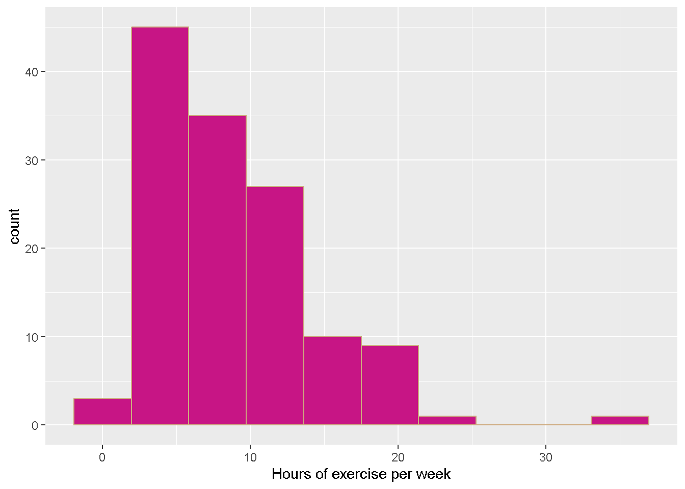
# measures of center
mean(stat113$Exercise)
## [1] 8.450382median(stat113$Exercise)## [1] 7# measures of spread
sd(stat113$Exercise)## [1] 5.464872# five number summary (and extra)
summary(stat113$Exercise)## Min. 1st Qu. Median Mean 3rd Qu. Max.
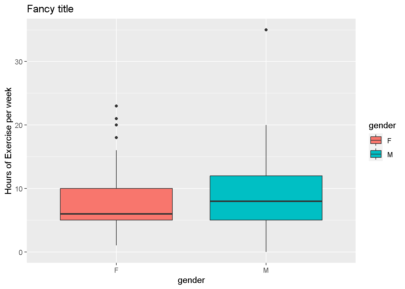
## 0.00 5.00 7.00 8.45 10.50 35.00# summary(stat113)- Visually compare reported exercise for males vs females.
ggplot(data = stat113,
       mapping = aes(x = Gender,
                     y = Exercise,
                     fill = Gender
                     )
       ) +
  geom_boxplot() +
  labs(y = "Hours of Exercise per week",
       x = "gender",
       fill = "gender",
       title = "Fancy title"
       )
Is there a relationship between amount of exercise and TV viewed? Use the appropriate plot to investigate this.
Do the “trends” differ by year?
ggplot(data = stat113,
       mapping = aes(x = TV, y = Exercise)
         ) +
  geom_point() +
  geom_smooth(color = "green", se = FALSE) +
  geom_smooth(method = "lm", color = "blue", se = FALSE)
## `geom_smooth()` using method = 'loess' and formula = 'y ~ x'
## `geom_smooth()` using formula = 'y ~ x'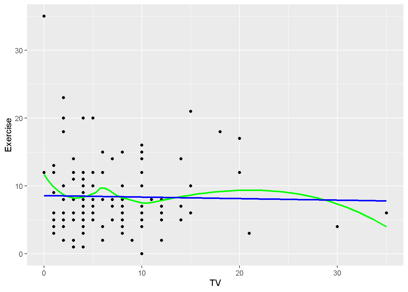
When we are done for the day, save your R Markdown file, close your R project to save it (say “Save” when asked), and log out of your Session.