2 Basic Statistical Analyses in R
2.1 Overview
In this document we will go through some of the basics doing a statistical analysis in R.
2.2 Goals
- Learn a few basics of R and R Studio
- You will begin to develop good habits for directory and file management in R Studio
- Learn how to do some basic “Stat 113 type” statistical analyses while using R.
2.3 Data Overview
The dataset ipa_recipes_brewerfriend.csv contains data on over 10,000 homebrew beer recipes from the Brewer’s Friend site. It is a subset of from the following: https://www.kaggle.com/jtrofe/beer-recipes
The variables included in our version are:
| Variable | Description |
|---|---|
| Name | Name of the beer recipe |
| Style | The beer style (will be American IPA for all recipes in the data) |
| Size(L) | The size of the batch of beer (in liters) |
| OG | The Original (Specific) Gravity of the unfermented beer (FYI, unfermented beer is called wort) |
| FG | The Final (Specific) Gravity of the beer (i.e., after fermentation is complete) |
| ABV | The percent Alcohol Content By Volume |
| IBU | International Bittering Units - a crude measurement of the bitterness in a beer due to the amount of hops in it |
| Color | The color of the finished beer, according to the Standard Reference Metric (SRM). In general, higher values are associated with darker beers |
| BoilSize | The initial size of the boil (in liters) |
| BoilTime | The number of minutes the wort is boiled - typically 60 or 90 |
| Efficiency | A measurement of how much of the starch in the grains (or extract) is converted into sugars |
| BrewMethod | The method used to brew the beer: All Grain, Extract, or Partial-Mash. Of these, extract brewing is the method used by most beginners. |
The two specific gravities (OG and FG) are major measurements used by brewers to determine the alcohol content of a beer fermented from a particular wort (i.e., unfermented beer). For reference, water is deemed to have a density at specific gravity of 1.000.
2.4 Sample Data Analysis
2.4.1 Load Necesary Packages
One of the greatest features with R is that it has a huge number of custom built packages that can be used to help nearly any type of data. To gain access to these we move load the packages we will need for the analysis. This is done using the library() function.
library(readr)## Warning: package 'readr' was built under R version 4.2.32.4.2 Read in the Data
When structured nicely, Comma Separate Value files (.csv extension) are some of the easiest data to load into your R Environment. While we will discuss importing different types of data in more detail in the upcoming weeks, basic tidy tabular data stored in a csv file can be imported very easily with the `read_csv`` function.
ipas <- read_csv("data/ipa_recipes_brewersfriend.csv")## Rows: 10657 Columns: 12
## ── Column specification ────────────────────────────────────────────────────────
## Delimiter: ","
## chr (3): Name, Style, BrewMethod
## dbl (9): Size(L), OG, FG, ABV, IBU, Color, BoilSize, BoilTime, Efficiency
##
## ℹ Use `spec()` to retrieve the full column specification for this data.
## ℹ Specify the column types or set `show_col_types = FALSE` to quiet this message.The object you’ve created is data.frame (or, more specifically, a version of it called a tibble).
2.4.2.1 Exercises
- Run the following code chunk and look at the error message that is displayed in the console. With your neighbor, take a few seconds to discuss why it doesn’t work.
ipas <- read_csv("/home/iramler/stat_234/notes/data/ipa_recipes_brewersfriend.csv")Relative vs Absolute Paths: Data files have a name and are located in a folder. (A folders is the same a directory. You will see both of these names in common use.) The folder containing the file may be nested within another folder and that folder maybe in yet another folder and so on. The specification of the list of folders to travel and the file name is called a path. A path that starts at the root/home folder of the computer is called an absolute path. A relative path starts at a given folder and provides the folders and file starting from that folder. Using relative paths will make a number of things easier when writing programs and is considered a good programming practice.
2.4.2.2 Variable types in R
In your environment, check out what type of variable each column of our data is stored as. Compare that to what you came up with earlier.
There are many different ways that R can store objects (called types, classes, or structures). Many of these have straightforward connections to concepts in statistics. (e.g., vectors are pretty similar to a variable in statistics, while a matrix can be thought of as a very crude looking data set) We will likely come across numerous types of objects throughout the semester and will introduce them as necessary.
2.4.2.3 Simple Graphics
We’ll spend a bit of time this semester learning about graphics using the ggplot2 package. For now, we’ll just make a few basic plots using that package. Start by adding a line to load the ggplots2 package your R chunk where we loaded the readr package. (Then run that new line of code.)
library(ggplot2)## Warning: package 'ggplot2' was built under R version 4.2.32.4.2.4 Exercises
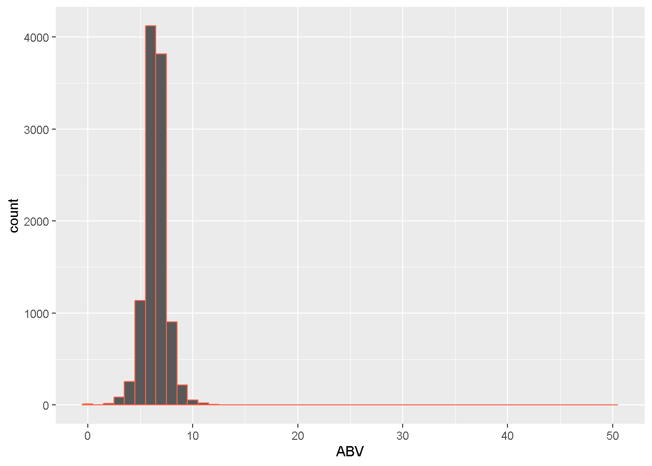
- Create a display of the alcohol content (ABV) in American IPAs.
ggplot(data = ipas,
       mapping = aes(x = ABV)
       ) +
  geom_histogram(binwidth = 1, color = "tomato")
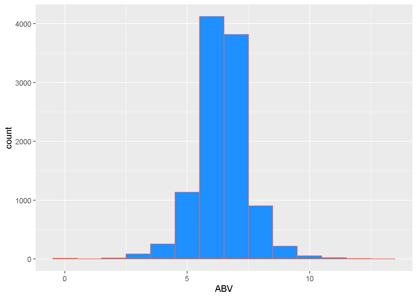
Remove beers with unrealistic ABVs.
library(dplyr)## Warning: package 'dplyr' was built under R version 4.2.3##
## Attaching package: 'dplyr'## The following objects are masked from 'package:stats':
##
## filter, lag## The following objects are masked from 'package:base':
##
## intersect, setdiff, setequal, unionipas <- filter(ipas, ABV < 15) # keeps only beers with ABV less than 15ggplot(data = ipas,
mapping = aes(x = ABV)
) +
geom_histogram(binwidth = 1,
color = "tomato",
fill = "dodgerblue"
)
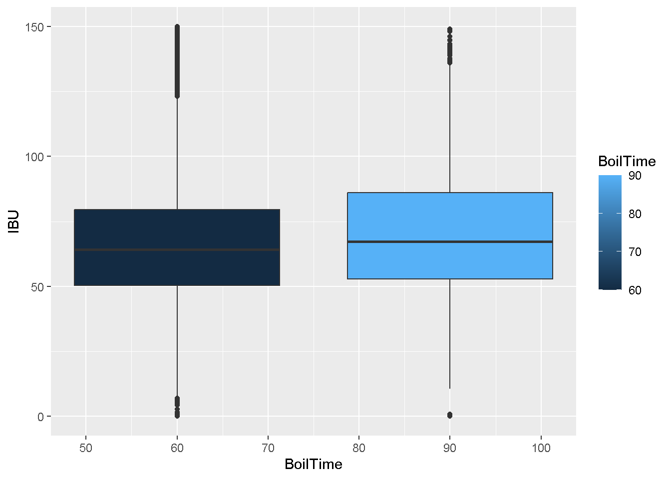
- Create a display comparing the bitterness (measured in IBUs) for 60 vs 90 minute boils.
Keep only beers with legit IBU (less than 150)
ipas <- filter(ipas, IBU < 150)ggplot(data = ipas,
mapping = aes(x = BoilTime,
y = IBU,
fill = BoilTime,
group = BoilTime
)
) +
geom_boxplot()
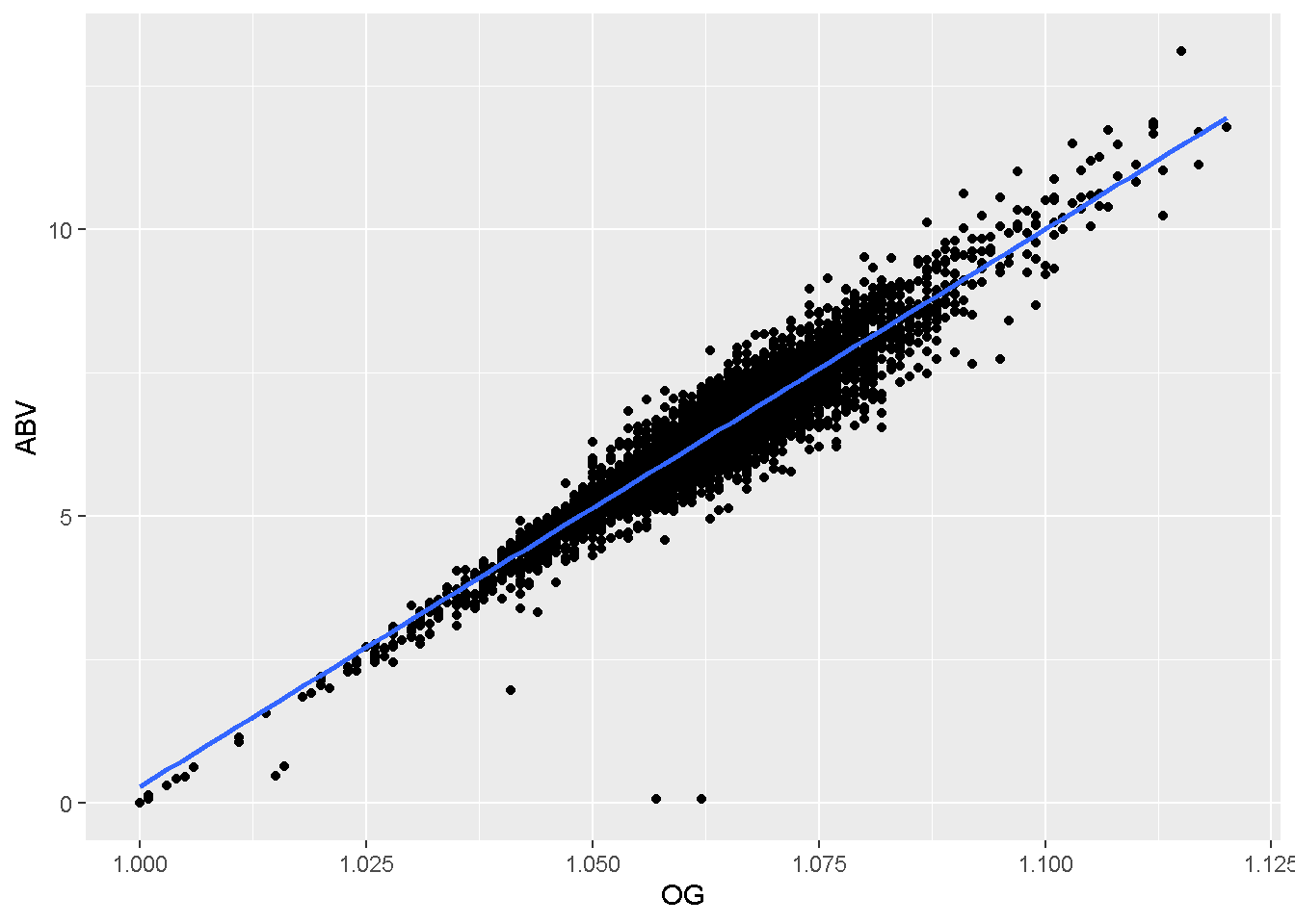
- Create a display to visualize the relationship between Original Gravity (OG) and Alcohol Content (ABV).
ggplot(data  = ipas,
       mapping = aes(x = OG,
                     y = ABV)
       ) +
  geom_point() +
  geom_smooth(method = 'lm')
## `geom_smooth()` using formula = 'y ~ x'
2.4.2.5 Statistical Inference (and basic modeling)
Many of the basic statistical inference procedures (both confidence intervals and hypothesis tests) have functions available in R without having to install or load any additional packages. Here are a few of the more common methods
| Method | Function |
|---|---|
| single proportion | binom.test (exact test - preferred) or prop.test (normal approximation) |
| difference in two proportions | prop.test or chisquare.test |
| single mean | t.test |
| difference in two means - independent samples | t.test |
| difference in two means - paired samples | t.test |
| comparing multiple means | aov and TukeyHSD (post-hoc comparisons) |
| correlation | cor and cor.test |
| linear regression | lm |
| logistic regression (STAT 213 topic) | glm |
In addition to the above, there are thousands of other methods available in R. Many of these are in community built packages.
Other functions you might find useful when doing statistical analyses are summary, with, and several from the broom package - tidy, glance, and augment. You will also want to become familiar with nicer ways to display tables of data/results when you “knit” an R Markdown. We’ll see this in more detail when we get closer to the first project, but will use the kable function from the knitr package today as a quick preview.
A Note on randomization/resampling based inference: Resampling based inference (e.g., bootstrap confidence intervals and randomization hypothesis tests) are often failry easy to do in R too. Some of the more standard style (similar to what those in STAT 113 with Drs. Robin and Patti Lock see) have pre-made functions. (See the
bootpackage for examples.) Non-standard resampling based inference is doable too - it just takes a little extra programming. Time permitting, we will see some basic approaches to writing our own resampling based inference programs. (Those that have taken CS 140 will also recognize the use of for-loops during that unit.)
2.4.2.6 Exercises
- Consider the ABV of American IPAs.
- Construct a 95% confidence interval for the mean ABV. Do so by providing a numeric vector of the data.
t.test(ipas$ABV)##
## One Sample t-test
##
## data: ipas$ABV
## t = 622.2, df = 10201, p-value < 2.2e-16
## alternative hypothesis: true mean is not equal to 0
## 95 percent confidence interval:
## 6.384824 6.425180
## sample estimates:
## mean of x
## 6.405002- Construct a 90% CI for the mean ABV.
t.test(ipas$ABV, conf.level = 0.9)##
## One Sample t-test
##
## data: ipas$ABV
## t = 622.2, df = 10201, p-value < 2.2e-16
## alternative hypothesis: true mean is not equal to 0
## 90 percent confidence interval:
## 6.388068 6.421936
## sample estimates:
## mean of x
## 6.405002- Construct a 98% CI for the mean ABV while using the
withfunction to pass the data in as an argument. Store the result as an object and investigate it using thetidyfunction from thebroompackage. After that, extract just the lower bound of the CI and round it to 2 decimal places.
# construct the 98% CI
abv_ci98 <- with(ipas, t.test(ABV, conf.level = 0.98)  )

# access the tidy function from the broom package
abv_ci98_tidy <- broom::tidy(abv_ci98)

# extract lower bound and round it to 2 decimal places
round( abv_ci98_tidy$conf.low , digits = 2)
## [1] 6.38- Is there a statistically significant difference in the IBUs for 60 minute vs 90 minute boils? Report just the results in a
tidytibble.
ibu_60_vs_90 <- ipas %>%
                with(t.test(IBU ~ BoilTime) ) %>%
broom::tidy()- Are there any statistically significant differences in Color for the three different brew methods? Check out the results (after fitting the appropriate statistical model) using each of the following functions:
summary,glance, andtidy.
color_anova <- ipas %>%
                with(aov(Color ~ BrewMethod))
summary(color_anova)
## Df Sum Sq Mean Sq F value Pr(>F)
## BrewMethod 3 790 263.21 10.01 1.38e-06 ***
## Residuals 10198 268054 26.28
## ---
## Signif. codes: 0 '***' 0.001 '**' 0.01 '*' 0.05 '.' 0.1 ' ' 1broom::glance(color_anova)## # A tibble: 1 × 6
## logLik AIC BIC deviance nobs r.squared
## <dbl> <dbl> <dbl> <dbl> <int> <dbl>
## 1 -31149. 62308. 62344. 268054. 10202 0.00294broom::tidy(color_anova)## # A tibble: 2 × 6
## term df sumsq meansq statistic p.value
## <chr> <dbl> <dbl> <dbl> <dbl> <dbl>
## 1 BrewMethod 3 790. 263. 10.0 0.00000138
## 2 Residuals 10198 268054. 26.3 NA NA- Use OG and FG to predict the ABV of an IPA.
abv_lmod <- ipas %>% with(lm(ABV ~ OG + FG))- Use the
knitrpackage and thekablefunction to construct tables of your results (from thetidyresults). Round all digits to 3 places and provide a brief, but informative caption. Run the chunk to see what it looks like. At the end of this tutorial, we will knit our R Markdown file as an HTML page and see what the table looks like in the resulting document.
abv_lmod_tidy <- broom::tidy(abv_lmod)

knitr::kable(abv_lmod_tidy, digits = 3, caption = "Linear Model results using OG and FG to predict alcohol content (ABV).")| term | estimate | std.error | statistic | p.value |
|---|---|---|---|---|
| (Intercept) | -1.206 | 0.189 | -6.391 | 0 |
| OG | 131.040 | 0.090 | 1455.103 | 0 |
| FG | -129.836 | 0.238 | -544.638 | 0 |